Difference between revisions of "Virtual society:results"

Revision as of 12:34, 3 November 2008

Virtual society | Virus spread | Literature | Version
Data | Model | Results

hidden contents

We are reporting here some selected results describing properties of our Basic Virtual Society model. In such a system various ranges of quantitative analysis can be considered. However, we focus here on the features essential for ongoing epidemiological and transportation studies, as well as on the planned future investigations. Since the methods used for recreation of a given social nodes, e.g. schools and workplaces are in principle similar, we limit the description here only to one selected type of network structure.

Basic Virtual Society - population and location of households

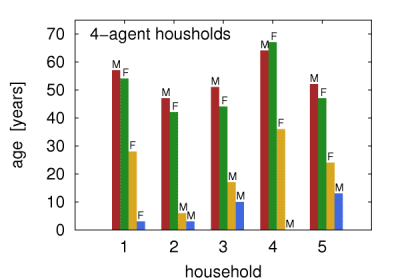
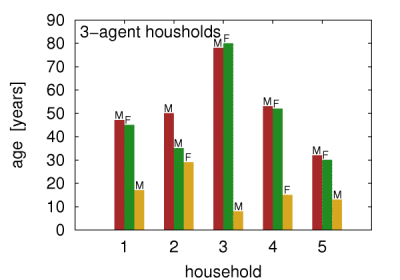
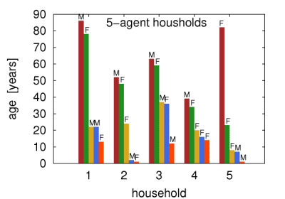
The obtained population of households reproduced the actual statistics obtained from the NCB. In particular, the number of inhabitants per km2 differs by less than 20 individuals from the values obtained from LandScan, and the size distribution of the households, the distribution of the age difference in couples/parents, the distribution of children number in households, and the distribution of the parents' age are all also well reproduced. Example 2,3,4, and 5-agent households are presented in Figures 1a-d.

Fig.1a:Example of virtual households created in this work. M and F symbols correspond to male and female agents, respectively

Fig.1c

Fig.1b

Fig.1d

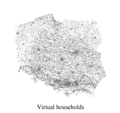
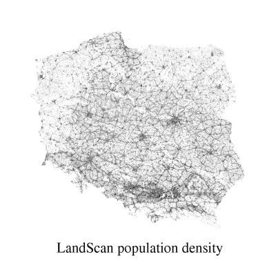
Comparison of real and virtual population densities is presented in Figures 2a,b.

Fig.2a: Visual comparison of real population density in Poland (from the LandScan data), and virtual population density represented by density of households. Both data sets were created with 1 km2 resolution.

Fig.2b

Both figures show smaller population density in the NW and NE parts of the country, very high population density in the central-southern region of the country, and in some small concentrated areas corresponding to bigger agglomerations. The biggest conurbation areas are that of the capital city in the central-eastern part of the country, and a highly populated, and industrialized areas in the South. These are the most characteristic features of population density in Poland, and they are accurately well reproduced by our virtual society modeling simulations.

Distance to institution statistics

Once the BVS is created and some basic infrastructure networks such as schools or workplaces are added, it is possible to extract the required population statistics. This would serve as a verification and validation of the model, provided that the corresponding statistical data are available.

Within the virtual society created so far, the mean distances for pupils and students to travel to their respective schools, colleges, as well as for workforce to travel to their workplaces were calculated. In each case the distance was calculated just as a Cartesian distance between two points. The appropriate mean distance statistics were calculated at a commune, poviat, or voivodeship resolutions.

Mean distances from households to schools

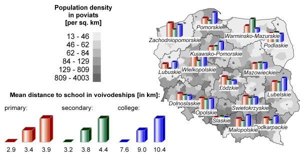
The results obtained for the three educational levels (primary and secondary schools, colleges) are presented in Figure 3 at a voivodeship resolution, within the context of population density in poviats.

Fig.3:Mean distance from household to school (primary, secondary, or college) in voivodeships (bars), and mean population density in poviats (hatch-map).

Typically, the more densely populated a given voivodeship is, the more schools are available and hence, the shorter is the mean household-school distance. Thus, the shortest distances to travel have pupils in Slaskie voivodeship in the South of Poland. This voivodeship is characterized by a rather uniform, high population density. The medium mean distances in Mazowieckie voivodeship (the one that includes the capital city of Warsaw) is the result of relatively short distances in highly populated, and abundant in schools, capital city, and relatively low density population and poor school availability in the surrounding communes.

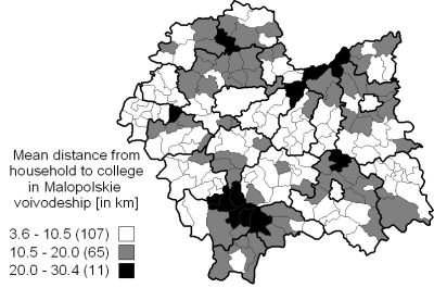
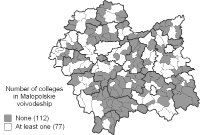
As a more detailed test case we chose Malopolskie voivodeship located in the southern Poland, mostly because of the surveillance statistics availability for this region^[1][2]. Figures 4a-c show colleges availability in communes of Malopolskie voivodeship.

Fig.4a:The average time necessary to get to the college in villages or cities (data from the work of Guzik^[1]).

Fig.4b:The average household-college distance in communes obtained using the model described in this work.

Fig.4c:The presence of schools in the communes (data from NCB).

Figure 4a presents times necessary to reach the college in Malopolskie voivodeship in years 1998-1999. The original data^[1] in the finer, village resolution were projected on the commune territories. This survey relates to the timing of getting to schools and divide travel time into three categories: short - up to 45 minutes, long - between 45 minutes and 90 minutes, and very long - above 90 minutes.

Figure 4b contains the data obtained from the model described here, and presents the mean distance from household to college in each commune. Finally, Figure 4c shows the presence of schools in each commune (grey fields mark the communes without any colleges).

One should note, that no complete correlation between time statistics^[1] and distance statistics from this work, is possible, because the latter does not yet account neither for any exact road network, nor for the transport timetable, while the former^[1] provides a detailed and extensive study of the exact travel times involved in educational availability in Malopolskie voivodeship. Nevertheless, a qualitative correlations are well reproduced, despite the presence of only Cartesian distance travel paths implemented so far.

Figure 4b marks out five regions of rather poor school availability, expressed in long household-college distances. In the case of the South-East and South region, the explanation may be the lack of schools in these regions shown in Figure 4c. This pattern is also visible in Figure 4a in the case of south-eastern region of Malopolskie voivodeship. The North and North-Eastern regions of long household-college distances are also pointed out as the regions characterized by long time necessary to reach the school. There is also a small North-West region visible in all three figures.

Mean distance to RSU

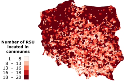
As we said, the addition of the subsequent RSUs was constrained to the minimal distance of 2 km between the units. Consequently, the maximum number of the located units in any commune (see Figure 5) corresponds to the area of that commune. Therefore, Figure 5 reflects also the area size distribution of communes in the whole country.

Despite the high numbers of RSUs, the regions of northern and western Poland (described by a low population density and relatively big areas of the constituting communes) are represented by the big mean distances to the rescue unit, as shown in Figure 6.

Fig.5: Maximal number of the RSUs located in particular commune.

Fig.6: Mean distance between a household and a rescue unit in a commune when maximum number of RSUs is placed in the commune.

Simplified economic analysis of the RSU system

Based on the models described so far, it is possible to carry out the preliminary economic analysis of the geo-referenced structure of RSUs distribution.

The most important factors that need to be balanced are the benefits related to a decrease of the mean distance between RSU and household, and the costs of creating any additional RSU in a commune. However, due to the inhomogeneous structure of the population density, it is not a straight forward task to correctly estimate general benefits of establishing another RSU in any commune.

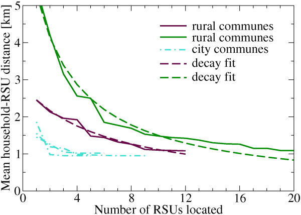
The mean distance from a household to the closest unit as a function of the number of RSUs in a commune is described here by a decaying function (named herein D). Function D is hyperbolic, since the mean distance to RSU is inversely proportional to the number of located RSUs. It also depends on a given commune topology. The following factors, among others, strongly affect the D-function: commune type (village, city, city-village), area of the commune and population density. Selected cases of D-function, presented as fits to the data, are shown in Figure 7.

Fig.7:Examples of different decay character of the mean distance from household to rescue unit versus number of rescue units. Fits presented in the plot regard only the case of villages.

A good measure of the non-linearity of the function in this case is a RMSD (Root Mean Square Deviation) calculated between the linear function fitted to the initial and final point of the decay, and the decay data. Initial point's coordinates are defined by the mean household-RSU distance at one RSU located, final point's - by the mean household-RSU distance at the maximum number of RSU located. When RMSD values are small, any addition of a rescue unit in the commune results with the significant improvement of the accessibility to the RSUs. When RMSD values are high, only few initial rescue units are beneficial because adding another RSU does not change much the mean distance to RSU.

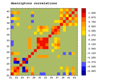
One can search for correlations between communes' descriptors, namely population and area statistics, and D-function properties in order to establish possible commune clusters. The proposed descriptors, and values used to characterize the D-function are listed in Table 1, below.

The correlation function may constitute an efficient analysis tool for a proper assignment of similarity among many communes. However, the set of proposed in this work communes' descriptors is not significantly correlated with the character of a D-function, namely it is not possible to deduce the economic properties of adding new RSU. However, we believe, it will reveal its usefulness in a further analysis. In the case of RSU, the correlation matrices indicate that the direct studies of a D-function might be a proper source of knowledge for such economic assessments.

The correlations that we observed (see Figure 8) show, that there is no significant correlation between the general statistical properties of communes of the same type and the decreasing distance to RSU due to increased number of RSUs.

Fig8a: Correlation matrices. For the sake of clarity, correlation values lying in the range [-0.370;0.370] are colored uniformly. The indices correspond to the properties given in Table 1.

Fig8b

References

1. ↑ ^{1.0 1.1 1.2 1.3 1.4} GUZIK R, Wybrane problemy badawcze geografii spolecznej w Polsce, Kat. Geogr. Ekonom. Uniw. Gdanskiego, Gdynia, 2001, chapt. Dostepnosc szkolnictwa sredniego a szanse zyciowe w obszarach wiejskich, pp. 215-224.
2. ↑ GUZIK R, Access to education and the knowledge-based economy in Poland: The regional perspective, in The Annual Anglo-Polish Colloquium "The Knowledge-Based Economy in Central and East European Countries: Exploring the New Policy and Research Agenda", SSEES-UCL, London., 2003

-->