Research
</br>
GENETIC STUDIES
Alignment-free genome sequence analysis by the ISSCOR method
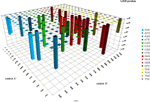
Synonymous codons do not occur at equal frequencies. Codon usage and codon bias have been extensively studied. However, the sequential order in which synonymous codons appear within a gene has not been studied until now. Here we describe an in silico method, which is the first attempt to tackle this problem: to what extent this sequential order is unique, and to what extent the succession of synonymous codons is important. This method, which we called Intragenic, Stochastic Synonymous Codon Occurrence Replacement (ISSCOR), generates, by a Monte Carlo approach, a set of genes which code for the same amino acid sequence, and display the same codon usage, but have random permutations of the synonymous codons, and therefore different sequential codon orders from the original gene. We analyze the complete genome of the bacterium Helicobacter pylori (containing 1574 protein coding genes), and show by various, alignment-free computational methods (e.g., frequency distribution of codon-pairs, as well as that of nucleotide bigrams in codon-pairs), that: (i) not only the succession of adjacent synonymous codons is far from random, but also, which is totally unexpected, the occurrences of non-adjacent synonymous codon-pairs are highly constrained, at strikingly long distances of dozens of nucleotides; (ii) the statistical deviations from the random synonymous codon order are overwhelming; and (iii) the pattern of nucleotide bigrams in codon-pairs can be used in a novel way for characterizing and comparing genes and genomes. Our results demonstrate that the sequential order of synonymous codons within a gene must be under a strong selective pressure, which is superimposed on the classical codon usage. This new dimension can be measured by the ISSCOR method, which is simple, robust, and should be useful for comparative and functional genomics. (more: http://www.sciencedirect.com/science/article/pii/S1631069108003223)
Correlating sequential and antigenic information
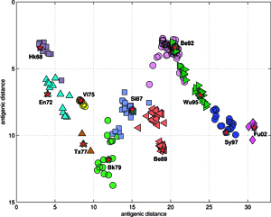
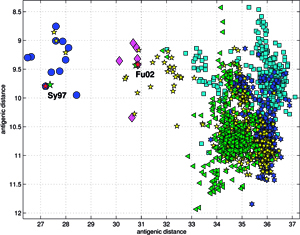
Analyses and visualizations by the ISSCOR method of influenza virus hemagglutinin genes of three different A-subtypes revealed some rather striking temporal (for A/H3N3), and spatial relationships (for A/H5N1) between groups of individual gene subsets. The application to the A/H1N1 set revealed also relationships between the seasonal H1, and the swine-like novel 2009 H1v variants in a quick and unambiguous manner. Based on these examples we consider application of the ISSCOR method for analysis of large sets of homologous genes as a worthwhile addition to a toolbox of genomics – it allows a rapid diagnostics of trends, and possibly can even aid an early warning of newly emerging epidemiological threats. Antibodies against hemagglutinin provide protective immunity to influenza virus infection, and the HA is therefore the primary component of influenza vaccines, and as the antigenic structure of HA changes significantly over time, vaccine has to be updated to ensure adequate efficacy against emerging viral variants. The WHO network of influenza centers routinely characterizes the antigenic properties of influenza viruses using inhibition assays, which combined with sequential data of variability in the antigenic HA-1 domain of the HA, are necessary to select strains for use in the seasonal vaccines. Smith et al. used antigenic data from 35 years of influenza surveillance between 1968 and 2003, with the resulting antigenic dataset consisting of a table of 79 post-infection ferret antisera by 273 viral isolates, and 4215 individual HA inhibition (HI) measurements, and then constructed an antigenic 2D map, to determine the antigenic evolution of influenza A/H3N2 virus, using projection from the obtained high-dimensional antigenic data hyperspace.
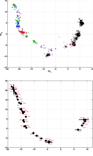
The accuracy of the predictions has shown that their map might serve as a possible target of an attempt to describe antigenic relationships on a basis of the ISSCOR descriptors. Partial least squares regression (PLS-regression) is a technique used to find relationships between two data sets (X and Y), utilizing a latent variable (LV) approach to modeling the covariance – possibly present in these two spaces. Rather than finding hyperplanes of maximum variance between the response and independent variables, like is the case in the PCA-regression, it finds a linear model by projecting the predicted variables together with the observables to a newly constructed space. In this way trying to uncover the multidimensional direction in the X space, that explains the maximum multidimensional variance direction in the Y space. Therefore, the PLS-regression of the antigenic cluster centers’ ISSCOR descriptors, on the 2D map of the Smith’s antigenic clusters, was performed, and the results are shown on the Figure above. The model utilizing six LVs was found to be optimal (RMS = 0.12), considering that the regression model obtained with only five LVs was not sufficient to achieve prediction errors small enough. Table II lists fifty of the most contributing ISSCOR variables used by each of the six LVs. At the bottom of each column there are values of explained variance for the ISSCOR descriptors [X-matrix], and the antigenic map’s cluster centers [Y-matrix]. It is noteworthy that only two major LV would already suffice to explain 95% of variance in Y space but at the same time all six LV are necessary to explain the respective variance in X – the 5th and the 6th LV are both contributing almost equally strong. The same PLS model was then used to project positions of H3N2 hemagglutinin strains isolated during each of the respective years (Fig. on the right). Of quite an interest is rather wide spread of the year’s 2005 sequences, some of which are apparently reversing the general trend observed earlier, and continued subsequently by the majority of strains isolated in the other 2003-2006 yearly seasonal clusters. (more: http://www.sciencedirect.com/science/article/pii/S1631069112000029)
Temporal and spatial evolution of the Influenza-A hemagglutinin genes
Two sets of the H3N2 influenza virus hemagglutinin (HA) sequences were collected – the set A comprising of 2217 full length HA gene sequences (1701 nucleotides each); and the set B of 1810 sequences of the HA-1 antigenic region of the H3N2 hemagglutinin gene (987 nucleotides each). The compositions of the sets A and B were almost entirely different as only two virus isolates were the same in both. The ISSCOR descriptors were calculated for these two sets of sequences, using. codon spacer values from 0 to 16, and creating two matrices (MA and MB) of 2217 and 1810 rows respectively, and 2448 columns each. It was observed that the G+C content in H3N2 hemagglutinin sequences of the set A decreased linearly over the period of 40 years, by approx. 5.93% – which corresponds to the changes in the relative ratios of all four nucleotides, although by different amount for each. The linear regression parameters of the equation Nucleotide_count = Pn * year + bn were PA = 0.9608 and bA = -1.3513 * 103; PC = -0.2751 and bC = 0.8903 * 103; PG = -0.8387 and bG = 2.0607 * 103; PT = 0.1463 and bT = 0.1148 * 103 – respectively for the A, C, G, and T nucleotides. This observation is consistent with the findings of Rabadan et al., who examined ratios of A, C, G and T in the PB1, PB2 and PA segments of genomes H1N1 and H5N1. For periods of up to 90 years, they found systematic and significant changes in GàA and CàT ratios in the both H1 and H5 cases, corresponding to hosts from which viral isolates were obtained – this was also usually associated with striking differences between sequence isolates of avian and of human origin.
Results of principal component analysis (PCA) for the matrix MA, are depicted on Figure at the left (the bottom panel). There is a clear timeline trend of the sequences from the years 1968-1970, which are located at the upper left corner, going down towards the minimum at about the years 2001-2002, and then up again to reach the years 2007-2008 at the end of the right arm of the curve. Therefore, to examine this trend more synthetically, the yearly clusters were considered separately for each year between 1968 and 2008. For each yearly cluster their centers, as well as the corresponding standard deviations, were calculated, and are shown. The horizontal and vertical bars are proportional in sizes to the respective standard deviations of PC-1 and PC-2 values. Noteworthy, there are three regions of rather increased variability: first – around the year 1968, then the years 2000-2003, and finally the year 2008, with some less diverse periods in between as well. It was found earlier, based on extensive analyses of influenza HA sequences of the H1 and H3 subtypes, that the evolution of H3N2 hemagglutinin included long intervals of mostly neutral sequence evolution without noticeable antigenic change showing an excess of synonymous over nonsynonymous substitutions, punctuated by shorter intervals of rapid evolution during which newly dominant lineages quickly displaced previously coexisting ones. The stasis intervals showed rather uniform distribution of replacements over the whole HA sequence’s length, not favoring epitope regions. The analogous PCA results for the matrix MB, showing 1810 data points, are depicted on the top panel, marking also members of the antigenic clusters, described earlier as forming WHO vaccine clusters. Of special interest is the location of the A/Fujian/411/2002 sequence on this plot (the red diamond at about PC1=5 and PC2=0) as this is the oldest of the six strains constituting the Fu02 cluster, and yet all remaining sequences of this cluster (each isolated in 2003) have their PC2 values below it. Holmes et al. concluded that one clade of H3N2 viruses present at least since 2000 had provided the hemagglutinin gene for all the H3N2 viruses sampled after the 2002–2003 influenza season, and that a reassortment event was the likely progenitor of the antigenicaly variant influenza strains that caused the A/Fujian/411/2002 epidemic of the 2003–2004 season. It is possible that a significant factor of such adaptation involved optimizing the functional compatibility of reassorting segments. Such a phenomenon might be a possible explanation why the lineage leading to the FU02 antigenic type did not dominate the viral population until a few years after its initial appearance, coincidental with an HA reassortment event.
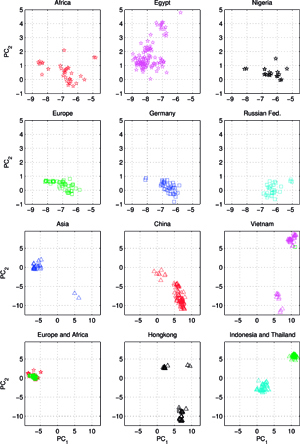
Another set C, comprising of 613 orthologous genes of the H5N1 avian flu virus’ hemagglutinin (HA), of 1707 nucleotides each – isolated from avian hosts during the 1996-2009 period – was acquired from NCBI in January 2010. All sequences were unique – in cases when two (or several) sequences were identical, only the earliest one was included. The ISSCOR descriptors were calculated for this set of sequences, using. codon spacer values from 0 to 16. The Figure on the right shows the PCA scatter plot of PC1 vs. PC2 for this set, divided for twelve territorial regions, characterized by the most numerous populations of isolates. Their plots are presented as separate panels, there are also separate panels showing remaining strains obtained from Africa, Asia and Europe. Already the analogous results for the A/H1N1 have shown some territorial clustering in several regions. In case of H5N1 the groupings are remarkably well defined and in many instances also rather well separated between themselves. This is especially evident for strains isolated in several Far Eastern, and South-East Asian countries: China, Vietnam, Hong Kong, Indonesia, and Thailand. On the other hand, isolates from Europe co-cluster together independently of their country of origin, which is also true for African and Middle-East countries – all of which form the large gathering at around PC1 = -3, and PC2 = 0 position. In roughly the same location there are also points for several Asian countries (all of which are different from the already mentioned five): Afghanistan, Pakistan, Bangladesh, India, Mongolia, Kazakhstan, and Japan. There are also two exceptions from Asia (well separated blue triangles in the panel "Asia") – one sequence from Japan (A/duck/Yokohama/aq10/2003, AB212280), and one from Myanmar (A/chicken/Pyigyitagon/204/2006, AB474081), both of them collocated together within the bottom cluster from China. The former H5N1 strain was isolated from duck meat processed for human consumption, imported to Japan from Shandong Province, China in 2003. That virus was antigenically different from other H5 viruses, including the Hong Kong H5N1 viruses isolated from humans in 1997 and 2003. The latter strain was isolated during the 1-st outbreak of bird flu in Myanmar in March 2006, and it was subsequently found to belong to the clade-7 (the WHO H5N1 evolution nomenclature) of the highly pathogenic avian influenza (HPAI). There is also one, rather unexpected case of the isolate from a Belgian crested eagle (A/crested_eagle/Belgium/01/2004, DQ182483; the green square, shown here for clarity at the edge of the top cluster in the panel "Vietnam"). On a closer examination this highly pathogenic H5N1 strain turned out to have been isolated from smuggled eagles, confiscated at the national airport, after an attempt to illegally enter them into Belgium from Thailand by a traveler. Phylogeography of H5N1 viruses was actively researched recently in the regions of Southeast Asia and Far East which were repeatedly subjected to outbreaks of bird flu in poultry, esp. in Vietnam, Thailand, and China, with conclusions rather similar ours, concerning the yearly origins and seasonal spread of the A/H3N2 viruses. Wallace et al. studied the geographic diffusion of H5N1 following the migration paths of the virus, by a way of a genetic phylogeography of H5N1’s HA and NA sequences, and shown that the Chinese province of Guangdong was the source of multiple H5N1 strains spreading at both regional and international scales. In contrast, Indochina appeared to be a regional sink, at the same time demonstrating bidirectional dispersal among localities within the region. They have shown further that the virus migration was filtered out at some international borders, like between China and Vietnam or Thailand, but not at e.g. the one between China and Japan. Their results were recently reanalyzed by Hovmoeller et al. who alleged that using a single tree, and a single optimization path, miss-estimates the frequency of transmission events, and moreover that the use of a single tree can fail to detect possible transmission events (more: http://www.actabp.pl/#File?./html/3_2014/441.html).
Improving the readability and an in silico automatic interpretation of Neighbor Joining phylogenetic reconstructions
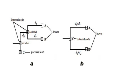
One of major drawbacks of traditional methods the phylogenetic trees reconstruction is that all molecular sequences are considered as leaves of the tree. Nodes in a phylogenetic tree can be divided in two types: [a] internal nodes, and [b] leaves. Internal nodes are sequences, which are distinct but have at least one offspring. In particular, an offspring can be an assemblage of internal nodes and/or leaves. Nodes with no offspring are ought to be presented as leaves, unfortunately, in traditionally build phylogenetic trees all sequences are treated as leaves, no matter if they have any offspring or not. Such trees treat internal nodes as auxiliary nodes to hold other nodes, or as information about potential ancestor sequence, which is not present in the analyzed set (Figure a on the left). This could pose a potential trap in designing algorithm analyzing evolutionary pathways, as one would expect ancestors to be closer to root than descendants (in the number of the edges between them). Only sequences on terminal branches (leaves), and the root are observed. All internal branches of the tree are not observed – if necessary, such sequences have to be estimated by the reconstruction (Ren et al.). Therefore, a possible other role of internal nodes in traditionally build trees might be to represent potential ancestor sequence[s]. This situation can happen only when all adjacent edges’ weights are greater than an unit distance – a necessary condition, as in any other edge weights’ configuration such an internal node will be just an ordinary auxiliary node. The ambiguity of leaves’ character, and internal nodes’ meaning in traditional phylogenetic trees contributes to difficulties in efficient analysis of evolutionary pathways in sillico. To alleviate this problem was the goal of the present study. The next section describes an algorithmic recipe, which considers character of all nodes in a traditional tree, and then attributes them with an appropriate role in a translated evolutionary tree (Figure b). In a schematic phylogenetic tree shown (panel a) typical reconstructed phylogenetic tree, which contains internal nodes without labels – written in Newick notationa as: ((A:d1, B:d2):d0, C:0); and (panel b) phylogenetic tree with all nodes labeled obtained from the tree in (a), written in Newick notation as: ((A:d0+d1, B:d0+d2)C:0); in both panels C is the ancestor of A and B.
Ever increasing amounts of genetic information stored in sequential databases require efficient methods to automatically reveal their phylogenetic relationships. We have implemented a framework for in silico unambiguous analysis of phylogenetic trees, based on information contained in tree’s topology, together with its branches length. The resulting, translated tree has all nodes labeled, with no constraints on nodes’ degree, and the subsequent finding of evolutionary pathways from the QPF-translated tree is robust and straightforward. Main features of the method are: small demands on computational time, and the ability to analyze phylogenies obtained prior to the proposed QPF analysis by any traditional tree-building technique. In the QPF approach edge’s weights distribution plays a crucial role as it is used to infer family character of nodes. In a perfect phylogeny’s tree all edge weights should be multiples of a unitary distance, so the pathway length between the nodes strictly represents distance between them. In a perfect phylogeny there are no two identical mutations at the same position. However, when analyzing a real sequence set such situation is not uncommon – the same mutations can occur at the same positions. Therefore, the edges’ weights distribution will be disturbed, and not all weights would be multiples of unitary distance. Such disturbed distribution depends on few factors. A bigger chance for a noisy tree occurs when: (i) the analyzed set consist a large number of sequences; (ii) sequences chain’s lengths are small; (iii) the number of characters which code each position in the chain is small; (iv) the mutations tend to be not distributed randomly throughout the chain (and also throughout a time domain – mostly due to biases in the time of samples isolation, and the numbers of isolated sequences). The proposed QPF algorithm translates a traditional phylogenetic tree, to a tree with all nodes labeled as to their phylogenetic character – in the resulting tree there are no auxiliary nodes, nor there are any nodes’ graph-theoretical degree constraints. Translated tree forms an adequate data structure, optimized for a quick evolutionary pathways finding. Therefore, although a resulting, translated tree might lose some information, as a side effect – should there be in particular any missing ancestors (not present in an analyzed sequences set), it is not necessarily a drawback, as for evolutionary pathways analysis only available sequences can be used anyway. The QPF is a robust, novel technique for an unambiguous labeling and analysis of phylogenetic trees generated by any traditional method of user’s choice. The assumption that the threshold value h is optimal when is set to the ½-unit distance, has confirmed the role of such threshold as a decision classifier distinguishing nodes of traditional phylogenetic tree into two classes – with a parent’s, or a child’s character. From a practical viewpoint, the proper choice of the h threshold value provide well over 95% accuracy, even for larger trees, despite a noise always present in traditionally generated trees' reconstructions.
In another extension of the classic NJ algorithm (which we've called NJ+), also enabling a correct handling of node assignments independently of node’s degree, the emphasis was given to a problem of correct handling sequences which might be missing in the analyzed set (the problem of missing ancestors). Again the NJ+ method reconstructs phylogenetic tree, by assigning the sequences with offspring as internal nodes, and the sequences without offspring as leaf nodes. In the resulting tree there are no constraints for the number of adjacent nodes, which means that the solution tree needs not to be a binary graph only. The subsequent derivation of evolutionary pathways, and pair-wise mutations, are then an algorithmically straightforward, with edge’s length corresponding directly to the number of mutations. The performance of the NJ+ method was examined on some synthetically generated artificial data, and two real data sets (Tryponosoma cruzi, and influenza 2009 pandemic virus hemagglutinin of H1N1). The performance tests on artificial and real data sets confirmed that the NJ+ method reconstructs trees with higher accuracy than the classic NJ algorithm. Obtaining evolutionary pathways and pair-wise mutations from the tree is straightforward, to facilitate further phylogenetic analyses. Additionally, other tree reconstruction algorithms can be extended in the proposed manner, to also give unbiased topologies.
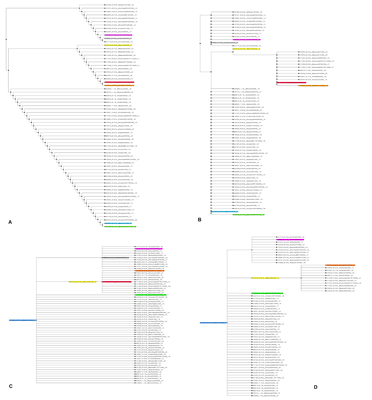
In order to illustrate the problem of inadequacy of existing phylogenetic trees to cope with ancestor sequences producing multiple (that is not binary) offspring, a small fragment of just few branches (67 sequences total) was culled from a large tree for the 2009 pandemic H1N1 virus hemagglutinin. The input tree, built from 3243 unique sequences of 1701 nucleotides each, contained many places where it was clear that respective mother sequences had multiple offspring (in the most striking case 41 unique daughter sequences). Each offspring sequence was distinct, and differed by just a SNP from its ancestor – therefore there were no ambiguity as to their respective ancestry. The trees, reconstructed for this small set of 67 sequences, by the NJ-classic algorithm, and by our modified NJ+ approach are presented on the Figure at the left (panel A: NJ-classic cladogram; panel B: NJ-classic phylogram; panel C: NJ+ cladogram; panel D: NJ+ phylogram). In the NJ-classic tree there were 133 nodes, and in the NJ+ tree – 67 nodes (every NJ+ node was labeled). The drawback of binary constraint of the NJ-classic is well observed in NJ-classic cladogram (panel A). It can not be as clearly observed in the NJ-classic phylogram (panel B) as distances between the respective auxiliary internal nodes are zero. However, because of binary limitations in the NJ-classic tree there are several edges distancing each mother and daughter pairs of nodes. In contract, the NJ+ reconstructions provide that there is always a spacer of exactly one edge between each daughter and mother sequences. (more: http://www.sciencedirect.com/science/article/pii/S1476927110000769)
Revisiting the founder mutation E391K of the influenza-A hemagglutinin from the H1N1 pandemic of 2009-2010
Inference of evolutionary pathways from traditionally generated phylogenetic trees is a difficult task for two reasons: first, in traditional phylogenetic tree all sequences are shown as leaves – the internal nodes are not attributed to any particular sequences. We can interpret such a tree as showing only sequences that had no descendants. However, it is more complicated, because even if there are sequences, which have their descendants in the set, they still will be shown only as leaves. Thus, the construction of traditionally generated tree does not augment finding of evolutionary pathways and interpretation. Secondly, many phylogenetic methods generate only binary trees, with all nodes of degree three or less. It is significant constraint, as generally any ancestor can have any number of immediate descendants. For a sequence that has more than two descendants, all of them will be shown on such a tree as an assembly of auxiliary internal nodes and leaves. Binary character of traditional tree is a consequence of clustering algorithms, which always merge pairs of sequences.
Keeping all the drawbacks in mind means that finding evolutionary pathways will grow to a problem of finding all ancestor-descendant pairs in a tree, which would require always running a check on all the nodes for every sequence – if anything, such an approach is computationally quite demanding. For these reasons we have proposed the QPF method (see above) to facilitate an unambiguous evolutionary pathway finding. Another problem, often present during phylogenetic analysis, is a possible absence of key sequences in the analyzed set. The problem of reconstruction accuracy and its dependence on sampling rates is well recognized in phylogenetic analysis, Two major underlying reasons are: the incomplete lineage sorting (ILS), and especially a possible absence in the analyzed sequences set some of key missing ancestors (MA). The problem of ILS received a lot of attention in the field of inferring species trees from gene trees. However, some issues leading to branches entanglement are also common in unraveling topology for a strain tree. In particular, when distances of sequence pairs are estimated within a set, it often happens that a given sequence might be less distant to some other sequence from an entirely different evolutionary pathway, than to its actual immediate ancestor, leading to its wrong branch assignment. The influence of MA would be especially evident while analyzing synthetic sequences sets – as the complete inheritance information contained therein can be unambiguously compared with resulting tree reconstructions.
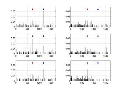
Two artifacts, both stemming from an increasing proportion of MAs in a set, are most troublesome. Artifact [a] concerns the orphaned sequences. When large fragments of evolutionary pathways are missing – leading to a decay of historical signal – then the only way to assign a pedigree of such an orphan is by linking it directly to a root of a whole tree (or sub-root of a branch). Which in turn can lead to [b] an overestimation of mutation rates at some branching node positions. A possible ratio of MAs for the whole 3243 sequences HA set can be only roughly guess estimated, although the collection of 2009 pandemic isolates is perhaps one of the best in a recent history. However, by comparing the results for the whole set, with the corresponding data for its subsets, an influence of MA ratio on mutation rates can be illustrated rather well. To this end we have performed series of multiple Monte Carlo (MC) experiments on this set, by randomly selecting just 10% of sequences each time, and then analyzing each subset for the number of detected mutations. The figure shows examples of mutation frequencies for the non-equivalent amino acids (as observed per nucleotide position, based on the change of character between four groups: non-polar, polar, acidic, and basic AA), carried on randomly drawn subsets (320 different orthologs each time).
The comparison of non-equivalent amino acid mutation frequencies per nucleotide position of 2009 pandemic H1N1 hemagglutinin, obtained for several, randomly drawn, subsets of 320 sequences, calculated on their Neighbor Joining trees is shown on the Figure at the right. The red diamond marks the mutation A716G, whereas blue circle the G1171A one. The vertical axis corresponds to observed mutation frequencies normalized per sequence. The HA-1 epitopic region spans 987 nucleotides, starting from the position 49, so the mutation G1171A lies slightly outside of it.
Phylogenetic analyses based on small to moderately sized sets of sequential data lead to overestimating mutation rates in influenza hemagglutinin (HA) by at least an order of magnitude. Two major underlying reasons are: the incomplete lineage sorting, and a possible absence in the analyzed sequences set some of key missing ancestors. Additionally, during neighbor joining tree reconstruction each mutation is considered equally important, regardless of its nature. Here we have implemented a heuristic method optimizing site dependent factors weighting differently 1st, 2nd, and 3rd codon position mutations, allowing to extricate incorrectly attributed sub-clades. The least squares regression analysis of distribution of frequencies for all mutations observed on a partially disentangled tree for a large set of unique 3243 HA sequences, along all nucleotide positions, was performed for all mutations as well as for non-equivalent amino acid mutations – in both cases demonstrating almost flat gradients, with a very slight downward slope towards the 3′-end positions. The mean mutation rates per sequence per year were 3.83*10^-4 for the all mutations, and 9.64*10^-5 for the non-equivalent ones.
We argue that tree reconstructions minimizing a number of spurious multiplication of a single “true” G1171A mutation (to the extent possible by the internal contradictions extant in an analyzed sets of sequences) are important for a better estimation of mutation rates. The actual composition of this set determines that there always will be at least one mutation on each of the 1226 positions, irrespective of the tree reconstruction method used. The mutable positions are therefore 72% of the gene length; while 28% are strictly conserved – a proportion in almost exact agreement with Eigen’s estimates for RNA viral evolution. The ratio of variable vs. hypervariable regions, however, depends on the tree reconstruction approach employed – approximately 40% of these 1226 mutations will have an amino acid changing character, although their exact number and the compositions are dependant to some extent on the reconstruction approach employed. Nevertheless, disentangling tree’s branches not only helps to eliminate spurious peaks of overestimated mutation rates, but it also makes possible to trace mutations occurring for the same codons – esp. of non-equivalent amino acid changes subsequent to a previous simple silent nucleotide mutations – both vital factors to consider. Moreover, such accumulation can lead to yet another phenomenon: of co-clustering several mutations within the same sub-clades, like e.g. the T1056C (G352, silent mutation, on 3rd codon position) with the C1656T (F552, silent, on 3rd position), or the T1408C (L470, silent, on 1st position) with the C1437T (N471, silent, on 3rd position). This might lead to forming a possible “foundation” for a subsequent non-reassortant genetic shift event, of the type recently sought experimentally by Imai's or Fouchier's groups, and then mathematically modeled by Russell et al. in a study of probabilistically estimated substitutions, leading possibly to more virulent strains. But even more important for such model predictions would be the ability to use data for time and location resolved evolution pathways with reasonably better levels of confidence, esp. as our estimated substitution rates for H1N1 pandemic, obtained through the disentangled three method, are of at least magnitude order lower than estimated earlier. (more: http://dx.doi.org/10.1016/j.ympev.2013.08.020)
Role of the host genetic variability in the influenza A virus susceptibility (a review)
The initial motivation for this review was an open question: Is susceptibility to severe influenza in humans heritable? – hard to answer, but not due to a lack of genotyping or analytic tools, nor because of insufficient evidence from severe influenza cases, but because of the absence of a coordinated effort to define and assemble cohorts of cases. Here we presented an update overview of the host variability of genes associated with flu infection, and discuss the possible influence of this variability on the severity of flu infection. Each virus-host interaction begins with entry of the virus into the host organism, and ends either in death of the individual or in elimination of the virus by the immune system. Evolution of the host–pathogen interactions yields variants in host genes, several of which are ultimately associated with bad or good prognosis following infection, while boosting the host’s future resilience towards given, specific strain subtype of the viral epitopes. Even if the severity of infection was mild and/or asymptomatic, these variants have been shown to be polymorphic in different human populations, which could be correlated with the different rates of morbidity/mortality from the influenza-A infectivity. Therefore, the answer to the initial question is positive, the susceptibility to severe influenza in humans is heritable.
On the other hand, it does not mean that all causes and variance in symptomatology and morbidity of flu infections have been discovered, or that they are only due to host genetic profile, but there are clearly several genes in the human genome that might have a direct impact on the course of influenza-A infections. In particular, when considering the ethnicity-derived genomic variance, some aspects of specific habitats and climates should not be neglected. In temperate regions the peak flu infectivity is felt predominantly during the winter months and epidemics recur with a highly predictable seasonal pattern. The studies using mouse-adapted strains of influenza virus, with experiments performed in the winter months yielded a transmission rate of 58.2%, yet of only 34.1% in summer. It has been hypothesized that possible causes of such seasonality include fluctuations in host immune efficiency mediated by seasonal factors such as melatonin and vitamin D levels; the changes in host behavior (school attendance, indoor crowding, air travel, etc.); but in particular environmental factors, including temperature, relative humidity, and the direction of seasonal winds movement in the upper atmosphere. The role of the South-East Asia region, in particular in countries spanning latitudes from subtropical at the south to high-mountainous at the north through several climactic zones, as spawning grounds of new flu strains is very well known, and a field of intense phylogeographical research. In contrast, the situation differs in the [sub]tropical regions, which experience influenza throughout the year, with somewhat increased incidence during rainy seasons. Such regions, like rainforests of equatorial Africa, or Amazonian regions of Brazil, Venezuela and Ecuador, are still potentially rich areas for a concerted efforts to connect the possible ethnic genomics factors in isolated communities, with the influenza-A prevalence and infectivity patterns.
Also, many factors can cause modifications in DNA (epigenetic modifications) that alter gene expression. Several studies support the theory of prenatal/childhood programming as origin of various adult diseases. Epigenetic modifications were described to explain adult disease in response to environmental modifications in prenatal or childhood. For example, Yang and Huffman (2013) showed that individuals who suffer some sort of nutritional privation during gestation tend to become obese adults. It can be thought that if the pattern of methylation that is programmed in one's genome during development can affect the way that individual will react to a diet as an adult, it might possibly affect the way immune-related genes are expressed during infections.
Very recently the work of Guihot et al. (2014) demonstrated some curious cases that impose more questions than answers. The authors have found biological markers that can predict whether an individual is more prone to suffer lethal consequences to influenza infection. However, the genetic variability that underlies such markers is not well understood – e.g., some of the markers indicated a "trapping" antibodies in the lungs for the lethal cases, whilst the survivors had the antibodies freed into a blood. In another recent study Worobey et al. (2014) have hypothesized that the high mortality during the 1918 Spanish flu pandemic among adults aged ~20 to ~40 years might have been due primarily to their childhood exposure to a heterosubtypic putative H3N8 virus – estimated as to have been circulating from ~1889–1900. All other age groups (except immunologically naive infants) were likely to be partially protected by childhood exposure to N1 and/or H1-related antigens. Such tenet poses immediate questions. What possible immunological mechanism[s] already described, might explain such an increase of mortality rates? Especially a mechanism of contrasting the H3 non-naïve young-adult Spanish flu victims (but putatively naïve towards H1 serotype), with infants – by definition naïve to all HA subtypes. In effect such a mechanism would require a convincingly plausible pathway[s] of suppressing immunity specifically by an action of H3-derived epitopes. One possible mechanism would be that the exposure to this putative H3N8 virus could have caused a methylation pattern in some genes, especially on some paths of immune response, and as consequence these patients had an extremely severe flu. Also, maybe not all individuals exposed to this virus developed the same methylation patterns and final supressions due to the genetic variability known to exist in human populations. The authors postulate that a mechanism akin to original antigenic sin (OAS, Francis T, 1960) may have interfered with immune responses in some of those infected in 1918, and peaked in those exposed previously to the 1889 virus. However, such hypothesis opens important questions about possible molecular and immunological mechanisms pertaining to the actual OAS phenomena “in action”. It is obvious that many more studies of this type will be necessary to better understand how the environment and host genetic variability affects the susceptibility to the influenza-A virus. The present review shows that both host genetic variability as well as environment are clearly factors of great importance to determine such susceptibility. (more: http://www.actabp.pl/#File?./html/3_2014/403.html)
EPIDEMIC SIMULATIONS
A virtual Polish society
The individual agent-based models (IABMs) are devised to describe explicitly the interactions among individuals and their environment, thus providing a process-oriented alternative to strictly analytical mathematical models. The construction of such models requires, however, a generation of the system of the, so called, software agents, as well as the geo-referenced network of public objects (like schools, factories, offices, hospitals, transportation systems, etc.), as well as with the selected elements of infrastructure. Due to high dimensionality of this virtual society (multiple agents operating on multiple contexts), the evolution of such system is typically performed using the stochastic Monte-Carlo methods. Moreover, sometimes even the preliminary creation of such complex system, mostly because of the scarcity of the real data, calls for the usage of stochastic methods. The issues involved in the construction of virtual society stem mostly from a need to recreate details of the information contained, usually buried in aggregated data as delivered by national census bureaus, and/or other such services. There is a need, then, to devise techniques allowing for either deconvolution of various sources of the aggregated data into their constituting components, or reconstruction of original data, by building geo-referenced software constructs, which can serve as a reasonable approximation of the missing data with detailed enough granulation.
As an example of application of the AB system devised here, the simple analysis of the school accessibility in Malopolskie voivodeship was performed, namely, the results obtained within the model described were collated with available statistical data. Although the quantitative calibration was not possible, qualitative correlation turned out to be noticeable. Another use of the model was to simplify analysis of the number and locations of rescue service units (RSUs) in local communes. Although it certainly requires a significant development, the model opens the way to a country-wide, immediate analysis of the effectiveness of possible location of RSUs. Based on the model system, a selected panel of statistical tests was used to verify and validate the assumed input criteria and boundary conditions, such as e.g. the accessibility of schools or the location of rescue service units.
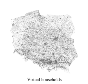
A particular emphasis was given to the contact patterns arising from daily commuting to schools or workplaces. The platform served as a base for further large scale epidemiological and transportation simulation studies. However, an application scope of the platform extends beyond the simulations of epidemic or transportation, and pertains to any situation where there are no easily available means, other than computer simulations, to conduct large scale investigations of complex population dynamics. While a virtual society exists only in the computer's memory, it reproduced the real Polish society rather well: consisting of individual (distinguishable) agents used to mimic the real society of 38 millions of citizens, each assigned to a certain, geo-referenced, household. Moreover, household inhabitants, depending on their age were either retired, employed or going to school (kindergarten, primary school, secondary school, college, university). All these basic relations were reflected in the virtual model as this virtual society was based on accessible census data. (more: http://jasss.soc.surrey.ac.uk/13/1/13.html)
Influenza epidemic spread simulation for Poland - a very large scale, individual based model study
The individual agent-based model (IABM) described above was used for studying the effects of influenza epidemic in large scale (38 million individuals) stochastic simulations, together with the resulting various scenarios of disease spread in Poland. Simple transportation rules were employed to mimic individuals' travels in dynamic route-changing schemes, allowing for the infection spread during their journeys.
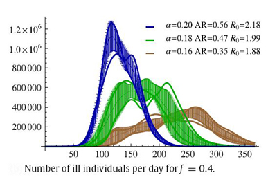
Parameter space was checked for stable behavior, especially towards the effective infection transmission rate variability. Following the assumptions employed in this work, a two-dimensional scan of the alpha and f parameters was performed in order to determine feasible scenarios of epidemic evolution. It should be noted, that the same R0 values may be obtained with different sets of alpha and f. In our research the R0 value varies from 1.44 to 2.42, which is a range comparable to other ranges studied in this field. In principle, R0 values are linearly related to alpha for each of the f values (R0 monotonically increases with alpha when other parameters, here f, are fixed), and therefore, the properties of the model system may be analyzed using alpha classification for each of the f ratios used. A series of possible epidemic courses for alpha ranging from 0.1 to 0.2 and for f taking values of 0.2, 0.4, 0.6, 0.8 and 1.0 were obtained by carrying out the simulations. In this parameter range we have encountered several similar R0 values which correspond to different epidemic courses. One can see that the definition of R0 does not fully account for the dynamically changing structure of the contact network or for the dynamic threshold of the "saturation" of the contexts with already infected or recovered agents. Therefore, the dynamics of the epidemic outbreak depends on the population, structure-type and infectiousness of the contexts. A rather atypical epidemic simulation run scenario for f=0.4 is depicted here as an example - atypical as for other f values epidemics run their courses much quicker (ranging from 100 to 250 days on average).
Although the reported model was based on quite simple assumptions, it allowed to observe two different types of epidemic scenarios: characteristic for urban and rural areas. This differentiates it from the results obtained in the analogous studies for the UK or US, where settlement and daily commuting patterns are both substantially different and more diverse. The resulting epidemic scenarios from these IABM simulations were compared with simple, differential equations based, SIR models: both types of the results displaying strong similarities. The pDYN software platform developed here was used in the next stage of the project, employed to study various epidemic mitigation strategies. (more: http://dx.doi.org/10.1016/j.physa.2010.04.029)
Probabilistic model of influenza virus transmissibility at various temperature and humidity conditions
Among the viruses that are spread efficiently by air, the influenza A virus causes one of the highest worldwide morbidity and mortality rates. However, there are still some factors related to its spread that have not been thoroughly examined and understood. In particular, the influence of weather conditions, such as air temperature and humidity, on the between-host transmission of this virus is not understood clearly, although many studies were carried out in the past. Thus far, the underlying reasons for the predominantly wintertime spread of influenza, significant for the understanding of its epidemiology and evolution, are still unexplained. Nonetheless, the seasonality of influenza epidemics is well characterized. In temperate regions influenza epidemics recur with marked regularity: in the northern hemisphere the influenza season spans period from November to March, while in the southern hemisphere epidemics last from May until September. Many theories have been proposed to explain this seasonal variation. Markedly different is influenza’s virus behavior in the tropics. Recently some results have provided direct experimental evidence of the major role of weather conditions in the dynamics of influenza transmission.
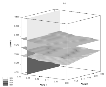
In particular, Lowen et al. used the guinea pig as a model host, and have shown that the efficiency of airborne influenza spreading depends upon both ambient relative humidity and temperature. However, these effects have not been satisfactorily recognized and quantified so far. Earlier we have presented a simple model of influenza transmission, which included some environmental variables. The transmissibility parameter occurring in that model was approximated for given conditions by comparing results of agent-based simulations with the actual experimental data. That approach had, however, quite substantial limitations regarding rather small size of the data set available. Consequently, the results were to some extent not entirely satisfying. In particular, the following problems were encountered while analyzing the model behavior at 20C: [a] the model failed to produce any statistically representative output that would be similar to the experimental results obtained for 35% humidity. The same concerns were also partially evident in the case of 20% humidity — unless an unexpectedly high and otherwise improper values of a certain ensemble-dependent parameters were assumed. [B] in the case of 50% humidity, for which a small infection rate occurred, that early model assigned the highest transmissibility. Moreover, the previous model provided ranges, rather than exact values, of parameters. More recently we proposed a probabilistic model, based on a different approach, which seems to be less sensitive to the size of the data set available. That statistical model of influenza transmission between individuals has also been derived from the results of the same laboratory experiments as before, which involved infecting guinea pigs with influenza at various temperatures and relative air humidity levels. The wide range of transmission rates in those experiments reflects the ensemble-independent phenomena. The correlations between most of our simulations and the experimental results were quite satisfactory. For several different conditions, we obtained transmissibility values which seem to be sufficiently accurate to provide a partial basis for an intended large-scale epidemiological study in a future. (more: http://dx.doi.org/10.1016/j.compbiolchem.2009.07.005)
