Difference between revisions of "Epidemics:ferguson2008"
(→Transmission level - parameters \alpha,\,\varepsilon,\,\beta,\,(\eta)) |
(→Prior level) |
||
| Line 63: | Line 63: | ||
That is prior distributions of all parameters, <math>\theta=(\mu, \sigma, \alpha, \beta, \varepsilon, \eta)</math> | That is prior distributions of all parameters, <math>\theta=(\mu, \sigma, \alpha, \beta, \varepsilon, \eta)</math> | ||
| + | |||
| + | Gamma distribution with mean <math>\mu=3</math> and standard deviation <math>\sigma=2</math> was used for the distribution of the duration times of infectious periods. Exponential distribution for <math>\alpha</math> and <math>\beta</math> were used | ||
== References == | == References == | ||
<references/> | <references/> | ||
Latest revision as of 15:06, 25 November 2008
| Virtual society | Virus spread | Literature | Version |
|---|---|---|---|
| Polish virtual society epidemics model | |||
| Guinea pigs epidemics model | |||
| Virus genetic evolution epidemics model | |||
Contents
Cauchemez et al Model[1]
An example of so called SIR (Susceptible, Infectious, Recovered) model.
Joint probability of observed (Y), unobserved variables ( ), and parameters (
 ) is given by:
 ,
,
where:
 ,
,  prior level (prior distributions of the parameters of the model).
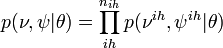 , transmission level
 , observation level
Y - indicator function:  (for ith, (
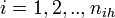 ) individual of ihth household (of size
  ) on jth day (
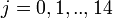 )), if clinical influenza was observed,
  otherwise.
  - all observations from household ihth, Y - observations from all households.
 - group of individuals at ihth household with at least 1 day of clinical influenza,
  - remaining members of the ihth household.
 - the 1st day of clinical influenza of ith individual in ihth household
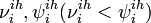 - unobserved variables corresponding to the start and the end of the infectious period for ith individual of ihth household
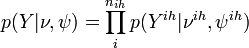
Observation level - parameters
![p(Y|\nu,\psi)=\left\{\begin{array}{ll}
1, & \textrm{if\;for\;all\;infected\;}i\,(i\in I): \nu_i\in [Z_i-3,Z_i] \land \nu_i < \psi_i\\
0, & \textrm{otherwise}
\end{array} \right.](/images/math/8/4/1/84177b6b9d5f65471dd2cf3d05c5bb89.png)
This level ensured that the unobserved data, , agreed with observed data, Y.
Transmission level - parameters 
The instantaneous risk of infection for an individual at time t in household of size n:
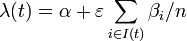 ,
,
where  - instantaneous risk of infection from the community and within household, respectively.
 - the group of infectives just before time t.
The duration of infectious period for ith infective  is taken from the gamma distribution with mean
  and standard deviation
  .
.
With the above, conditional on the date of the first infection  , we have (for the household):
![p(\nu,\psi|\theta)\,=\,\prod_{i\in I}\,d_{\mu_i,\sigma_i}(\psi_i-\nu_i)\prod_{i\in I-\{1\}}\,\lambda_i(\nu_i)\exp[-\int_{\nu_1}^{\nu_i}\lambda_i(t)dt]\,\prod_{s\in S}\exp[-\int_{\nu_1}^{15}\lambda_s(t)dt]](/images/math/0/7/8/078bfa5057da059d963a2770eb8eb196.png)
where I-{1} denotes infectives without the first infected
Prior level
That is prior distributions of all parameters, 
Gamma distribution with mean  and standard deviation
  was used for the distribution of the duration times of infectious periods. Exponential distribution for
  and
and  were used
References
- ↑ CAUCHEMEZ S, Carrat F, Viboud C, Valleron A J, Boelle P Y, A Bayesian MCMC approach to study transmission of influenza: application to household longitudinal data, Stat. Med., 23, (2004), p3469