Epidemics:guineapigs:model

Model's assumptions

We have formulated a discrete stochastic model based on the probability of infection. To estimate this probability, we apply a simple generalized linear model (GLM), with $f(p) = \ln(1-p)$ as the link function. This is a standard approach that has been successfully adopted in various related contexts for modeling influenza. The model starts from day zero, when all non pre-infected animals are healthy. For each consecutive day, we calculate the probabilities that each individual, among those not yet infected, will be infected on that day, and then we randomly check whether any of the possible infections actually happens. The infection history is subsequently updated, and the algorithm moves to the next day.

We assume the four following conditions:

1. The probability that the ith individual will be infected on a particular day (provided that it had not been infected previously) is

$p_i = 1 - \exp\left(-\gamma(T,H)\sum_j \alpha_{ij}\beta_j\right)$

where $\beta_j$ is a measure of virus concentration in the respiratory tract of the jth individual (decimal logarithm of the number of PFU in one ml of its nasal wash). The summation goes over individuals placed on the same and on adjacent shelves. Spatial coefficients $\alpha_{ij}$ are related to the probabilities that an aerosol drop, shed by the jth animal, will get to the ith guinea pig's cage. The coefficient $\gamma(T,H)$ reflects the dependence of the virus transmission rate on the air temperature (T) and relative humidity (H).

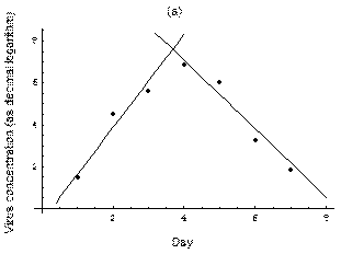
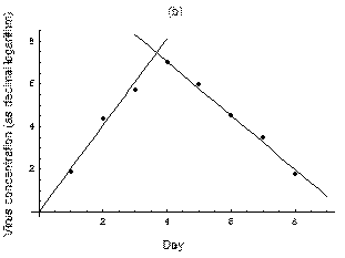
2. The course of influenza (virus concentration in nasal wash on the days subsequent to infection) depends only on the ambient temperature. Therefore, for each individual that became infected via air during the course of each particular experiment, the concentrations were assigned values reflecting the average case for that temperature. Table 1 shows the mean concentrations measured on particular days after infection, separately for each temperature. Functions comprising two linear pieces appear to be a reasonable guess, as shown in Figure 1.

tab.1: The average virus concentration in nasal wash of individual guinea pigs infected via air. For each individual, day 1 is the day when a measurable virus quantity first appeared in its respiratory tract

Day	1	2	3	4	5	6	7	8	9
Concentration, $T = 20^o$	1.52	4.52	5.63	6.89	6.06	3.26	1.88	-	-
Concentration, $T = 5^o$	1.91	4.40	5.72	7.02	6.01	4.54	3.52	1.77	-
Std. deviation square	0.40	0.59	1.26	0.32	2.38	1.44	3.18	2.34	-

Fig.1a

The two piecewise linear approximations of the infection course. For $20$ the best fit is $\beta(t) = 2.23 t - 0.61$ for the growing part and $-1.63 t + 13.62$ for the falling; for $5$ it is $2.03 t - 0.01$ and $-1.27 t + 12.13$ respectively. We assume $\beta = 0$ if the amount of virus is undetectable or zero

Fig.1b

This may be interpreted as a two-phase infection course: first, the virus concentration grows exponentially (the scale is logarithmic), and subsequently (mostly as a result of the immune system activation) it exponentially falls. The transition between phase 1 and 2 is always sharp.